Visualization is a helpful component in the process of interpreting results from high-throughput experiments, and can be indispensable when working with large data-sets. Within the GO, the "natural" visualization format is the Direct Acyclic Graph of a group of annotated sequences. In the DAG, each node represents a GO term. Arcs represent the relationships between the biological concepts. A problem when visualizing GO functional information of genomic data-sets is that these graphs can become extremely large and difficult to navigate when the number of represented sequences is high.

One of the functions of Blast2GO is the ability to display the annotation result of one or several sequences in the same GO graph. Within Blast2GO these graphs are called "Combined Graphs". This function generates joined GO DAGs to create overviews of the functional context of groups of annotations and sequences. Combined Graph nodes are highlighted through a color scale proportional to their number of sequences annotated to a given term. This confluence score (from now on denoted "node-Score") takes into account the number of sequences converging at one GO term and at the same time penalizes by the distance to the term where each sequence was actually annotated. Assigned sequences and scores can be displayed at the terms level.

Node Score

The node score is calculated for each GO term in the DAG and takes into account the topology of the ontology and the number of sequences belonging (i.e. annotated) to a given node (i.e. GO term). The score is the sum of sequences directly or indirectly associated to a given GO term weighted by the distance of the term to the term of "direct annotation" i.e. the GO term the sequence is originally annotated to. This weighting is achieved by multiplying the sequence number by a factor alpha [0, infinity] to the power of the distance between the term and the term of direct annotation (equation below). In this way, the node score is accumulative and the information of lower-level GO-terms is considered, but the influence of more distant information (i.e. annotations) is suppressed/decreased depending on the value of alpha. This compensates for the drawback of the earlier described method of simply counting the number of different sequences assigned to each GO-term. The alpha parameter allows this behavior to be further adjusted. A value of zero means no propagation of information and can be increased by raising alpha.

Graph Term Filtering

Combined graphs can become extremely large and difficult to navigate when the number of visualized sequences is high. Additionally, the relevant information in these cases is frequently concentrated in a relatively small subset of terms. We have introduced graph-pruning functions to simplify DAG structures to display only the most relevant information. In the case of the Combined Graph function, a cutoff on the number of sequences or the node-score value can be set to filter out GO terms. In this case the size of a graph is reduced without loosing the important information (i.e hiding tip and intermediate low informative nodes). 

This approach of graph-filtering and trimming is based on a combination of different scoring schemes. On the one hand, graph filtering can be based on the number of sequences assigned to each node, and on the other hand, a graph can be "thinned out" by removing intermediatealpha nodes that are below a given cutoff. The latter approach allows a certain level of details to be maintained while drastically reducing the size of the graph by removing "unimportant" intermediate graph elements. In this way, any large GO graph can be reduced by abundance and information content instead of simply "cutting through" the Gene Ontology at a certain hierarchical level or by the use of GO-Slim definitions. 

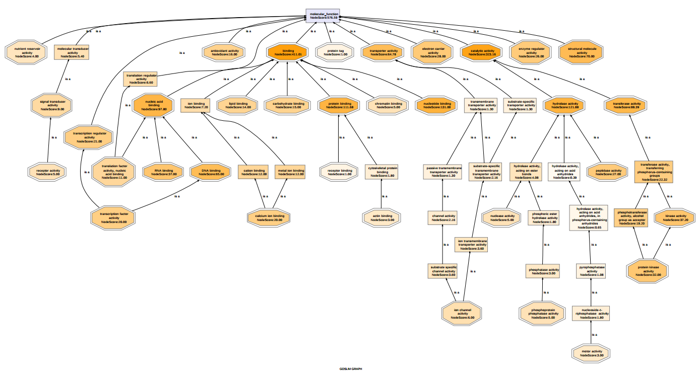
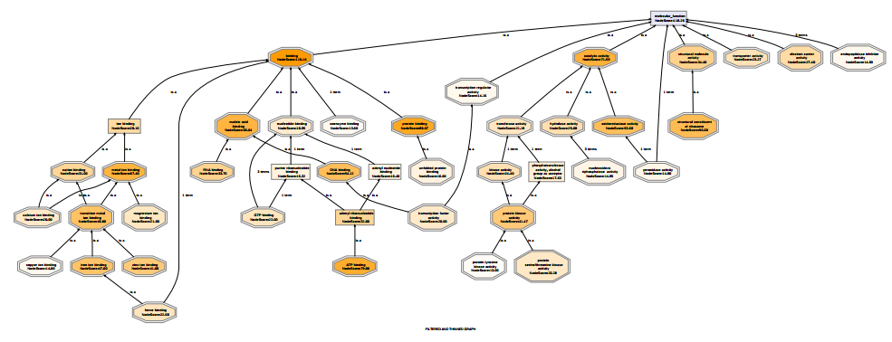
Below the molecular functions of 1000 sequences are visualized in 3 different ways. The first graph is unfiltered, the second graph shows the functional information after having applied a Go-Slim reduction. The third graph is filtered and thinned according to the number of sequences belonging to each GO-term and the node-score. All GO terms with less than 10 sequences were removed (tip nodes) and all the nodes with a node-score smaller than 12, applying an alpha of 0.4, were removed (intermediate nodes). This strategy allows the removal of terms that are less significant to a particular data-set while at the same time it maintains frequently present terms at lower levels of specificity.

Figure 1: Unfiltered Graph

Figure 2: Filtered Graph 1

Figure 3: Filtered Graph 2

Combined Graph Editor Sidepanel

General

This section controls the graph visualization within its area.

• Zoom
• Collapse All: The nodes will collapse and only the root will be visible.
• Expand All: The graph will expand to its entire size.
• Re-Layout: The whole graph will be re-scaled to adjust to the visualization area.

Find

Allows to search for GO IDs/ Terms/ Description in the Graph.

Node Info

Adjust the visible information in each node.

• GO ID: If checked the GO ID will be included in the node.
• GO Name: The GO Names are shown in the node.
• GO Description: The GO Description will be included in the node.
• Node score: The node score will be shown in the node.
• Sequence Names: The names of the sequences annotated annotated with this GO are shown (max. 15).
• Sequences: The number of sequences annotated with that particular GO will be displayed in the node.

Layout

• Edge Labels: When checked, the labels at the edges will be shown.
• Expand/Collapse Icon: If checked the ions that represent expand/collapse on the node are displayed.
• Only is a Relations: Only the is a relations between nodes will be displayed if the box is checked.
• Color
  • Ontology: All nodes will be colored according to the ontology category, Biological Process - green; Molecular Function - blue; Cellular Component - yellow.
  • White: The nodes will turn white.
  • By Node score: The higher the node score, the more intense is the color (orange).
  • By Sequence Count: Node color intensity will be proportional to the number of contributing sequences at the node.

Figure 5: Graph Legend that shows the graph shapes